5.8 Adding Fitted Lines from Multiple Existing Models
5.8.1 Problem
You have already created a fitted regression model object for a data set, and you want to plot the lines for that model.
5.8.2 Solution
Use the predictvals() function from the previous recipe (5.7) along with functions from the dplyr package, including group_by() and do().
With the heightweight data set, we’ll make a linear model for each of the levels of sex. The model building is done for each subset of the data frame by specifying the model computation we want within the do() function.
The following code splits the heightweight data frame into two data frames, by the grouping variable sex. This creates a data frame subset for males and a data frame subset for females. We then apply lm(heightIn ~ ageYear, .) to each subset. The . in lm(heightIn ~ ageYear) represents the data frame we are piping in from the previous line – in this case, the two data frame subsets we have just created. Finally, this code returns a data frame which contains a column, model, which is a list of the model outputs corresponding to each level of the grouping variable sex, female and male.
library(gcookbook) # Load gcookbook for the heightweight data set
library(dplyr)

# Create an lm model object for each value of sex; this returns a data frame
models <- heightweight %>%
  group_by(sex) %>%
  do(model = lm(heightIn ~ ageYear, .)) %>%
  ungroup()

# Print the data frame
models
#> # A tibble: 2 × 2
#>   sex   model
#>   <fct> <list>
#> 1 f     <lm>
#> 2 m     <lm>

# Print out the model column of the data frame
models$model
#> [[1]]
#>
#> Call:
#> lm(formula = heightIn ~ ageYear, data = .)
#>
#> Coefficients:
#> (Intercept)      ageYear
#>      43.963        1.209
#>
#>
#> [[2]]
#>
#> Call:
#> lm(formula = heightIn ~ ageYear, data = .)
#>
#> Coefficients:
#> (Intercept)      ageYear
#>      30.658        2.301
Now that we have the list of model objects, we can run the predictvals() as defined in 5.7 to get the predicted values from each model:
predvals <- models %>%
  group_by(sex) %>%
  do(predictvals(.$model[[1]], xvar = "ageYear", yvar = "heightIn"))
Finally, we can plot the data with the predicted values (Figure 5.24):
ggplot(heightweight, aes(x = ageYear, y = heightIn, colour = sex)) +
  geom_point() +
  geom_line(data = predvals)

# Using facets instead of colors for the groups
ggplot(heightweight, aes(x = ageYear, y = heightIn)) +
  geom_point() +
  geom_line(data = predvals) +
  facet_grid(. ~ sex)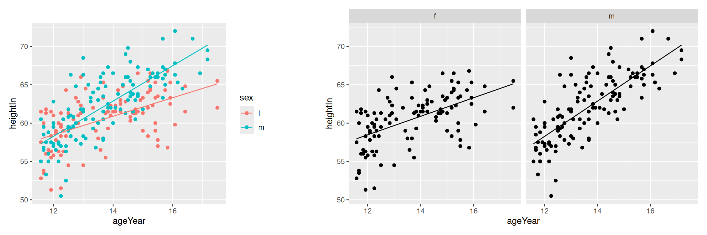
Figure 5.24: Predictions from two separate lm objects, one for each subset of data (left); With facets (right)
5.8.3 Discussion
The group_by() and do() calls are used for splitting the data into parts, running functions on those parts, and then reassembling the output.
With the preceding code, the x range of the predicted values for each group spans the x range of each group, and no further; for the males, the prediction line stops at the oldest male, while for females, the prediction line continues further right, to the oldest female. To form prediction lines that have the same x range across all groups, we can simply pass in xrange, like this:
predvals <- models %>%
  group_by(sex) %>%
  do(predictvals(
    .$model[[1]],
    xvar = "ageYear",
    yvar = "heightIn",
    xrange = range(heightweight$ageYear))
  )
Then we can plot it, the same as we did before:
ggplot(heightweight, aes(x = ageYear, y = heightIn, colour = sex)) +
  geom_point() +
  geom_line(data = predvals)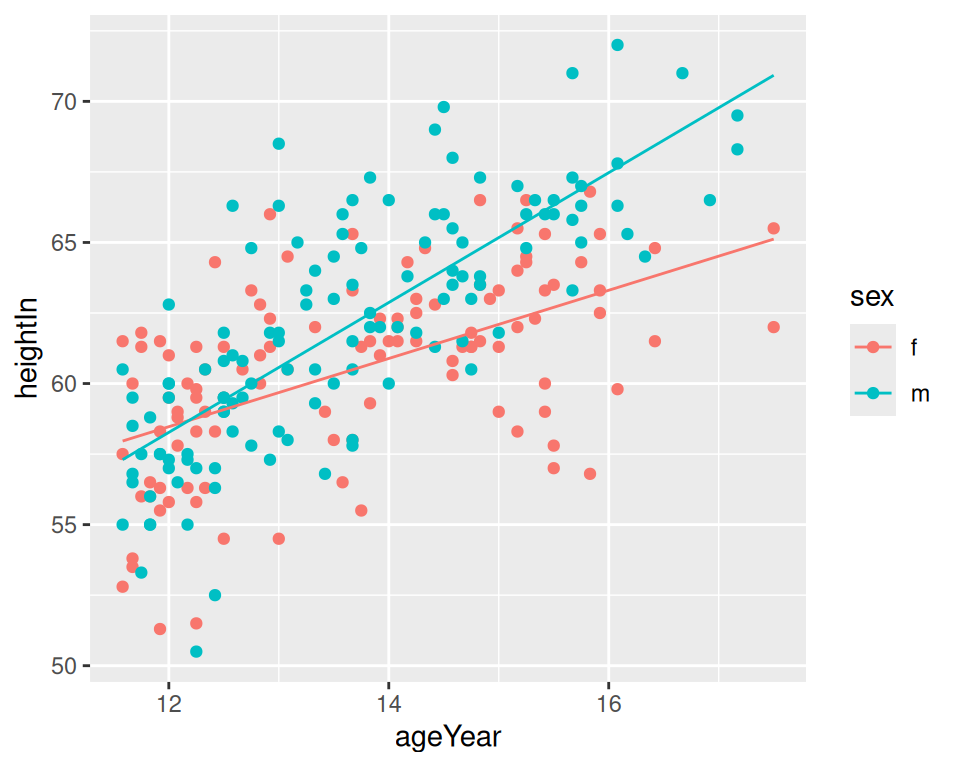
Figure 5.25: Predictions for each group extend to the full x range of all groups together
As you can see in Figure 5.25, the line for males now extends as far to the right as the line for females. Keep in mind that extrapolating past the data isn’t always appropriate, though; whether or not it’s justified will depend on the nature of your data and the assumptions you bring to the table.