15.17 Summarizing Data by Groups
15.17.2 Solution
Use group_by() and summarise() from the dplyr package, and specify the operations to do:
library(MASS)  # Load MASS for the cabbages data set
library(dplyr)

cabbages %>%
  group_by(Cult, Date) %>%
  summarise(
    Weight = mean(HeadWt),
    VitC = mean(VitC)
  )
#> `summarise()` has regrouped the output.
#> ℹ Summaries were computed grouped by Cult and Date.
#> ℹ Output is grouped by Cult.
#> ℹ Use `summarise(.groups = "drop_last")` to silence this message.
#> ℹ Use `summarise(.by = c(Cult, Date))` for per-operation grouping
#>   (`?dplyr::dplyr_by`) instead.
#> # A tibble: 6 × 4
#> # Groups:   Cult [2]
#>   Cult  Date  Weight  VitC
#>   <fct> <fct>  <dbl> <dbl>
#> 1 c39   d16     3.18  50.3
#> 2 c39   d20     2.8   49.4
#> 3 c39   d21     2.74  54.8
#> 4 c52   d16     2.26  62.5
#> 5 c52   d20     3.11  58.9
#> 6 c52   d21     1.47  71.8
15.17.3 Discussion
There are few things going on here that may be unfamiliar if you’re new to dplyr and the tidyverse in general.
First, let’s take a closer look at the cabbages data set. It has two factors that can be used as grouping variables: Cult, which has levels c39 and c52, and Date, which has levels d16, d20, and d21. It also has two numeric variables, HeadWt and VitC:
cabbages
#>    Cult Date HeadWt VitC
#> 1   c39  d16    2.5   51
#> 2   c39  d16    2.2   55
#>  ...<56 more rows>...
#> 59  c52  d21    1.5   66
#> 60  c52  d21    1.6   72
Finding the overall mean of HeadWt is simple. We could just use the mean() function on that column, but for reasons that will soon become clear, we’ll use the summarise() function instead:
The result is a data frame with one row and one column, named Weight.
Often we want to find information about each subset of the data, as specified by a grouping variable. For example, suppose we want to find the mean of each Cult group. To do this, we can use summarise() with group_by().
tmp <- group_by(cabbages, Cult)
summarise(tmp, Weight = mean(HeadWt))
#> # A tibble: 2 × 2
#>   Cult  Weight
#>   <fct>  <dbl>
#> 1 c39     2.91
#> 2 c52     2.28
The command first groups the data frame cabbages based on the value of Cult. There are two levels of Cult, c39 and c52, so there are two groups. It then applies the summarise() function to each of these data frames; it calculates Weight by taking the mean() of the HeadWt column in each of the sub-data frames. The resulting summaries for each group are assembled into a data frame, which is returned.
You can imagine that the cabbages data is split up into two separate data frames, then summarise() is called on each data frame (returning a one-row data frame for each), and then those results are combined together into a final data frame. This is actually how things worked in dplyr’s predecessor, plyr, with the ddply() function.
The syntax of the previous code used a temporary variable to store results. That’s a little verbose, so instead, we can use %>%, also known as the pipe operator, to chain the function calls together. The pipe operator simply takes what’s on its left and substitutes it as the first argument of the function call on the right. The following two lines of code are equivalent:
group_by(cabbages, Cult)
# The pipe operator moves `cabbages` to the first argument position of group_by()
cabbages %>% group_by(Cult)
The reason it’s called a pipe operator is that it lets you connect function calls together in sequence to form a pipeline of operations. Another common term for this is a different metaphor: chaining.
So the first argument of the function call is in a different place. So what? The advantages become apparent when chaining is involved. Here’s what it would look like if you wanted to call group_by() and then summarise() without making use of a temporary variable. Instead of proceeding left to right, the computation occurs from the inside out:
Using a temporary variable, as we did earlier, makes it more readable, but a more elegant solution is to use the pipe operator:
Back to summarizing data. Summarizing the data frame by grouping using more variables (or columns) is simple: just give it the names of the additional variables. It’s also possible to get more than one summary value by specifying more calculated columns. Here we’ll summarize each Cult and Date group, getting the average of HeadWt and VitC:
cabbages %>%
  group_by(Cult, Date) %>%
  summarise(
    Weight = mean(HeadWt),
    Vitc = mean(VitC)
  )
#> `summarise()` has regrouped the output.
#> ℹ Summaries were computed grouped by Cult and Date.
#> ℹ Output is grouped by Cult.
#> ℹ Use `summarise(.groups = "drop_last")` to silence this message.
#> ℹ Use `summarise(.by = c(Cult, Date))` for per-operation grouping
#>   (`?dplyr::dplyr_by`) instead.
#> # A tibble: 6 × 4
#> # Groups:   Cult [2]
#>   Cult  Date  Weight  Vitc
#>   <fct> <fct>  <dbl> <dbl>
#> 1 c39   d16     3.18  50.3
#> 2 c39   d20     2.8   49.4
#> 3 c39   d21     2.74  54.8
#> 4 c52   d16     2.26  62.5
#> 5 c52   d20     3.11  58.9
#> 6 c52   d21     1.47  71.8
Note
You might have noticed that it says that the result is grouped by
Cult, but notDate. This is because thesummarise()function removes one level of grouping. This is typically what you want when the input has one grouping variable. When there are multiple grouping variables, this may or may not be the what you want. To remove all grouping, useungroup(), and to add back the original grouping, usegroup_by()again.
It’s possible to do more than take the mean. You may, for example, want to compute the standard deviation and count of each group. To get the standard deviation, use sd(), and to get a count of rows in each group, use n():
cabbages %>%
  group_by(Cult, Date) %>%
  summarise(
    Weight = mean(HeadWt),
    sd = sd(HeadWt),
    n = n()
  )
#> `summarise()` has regrouped the output.
#> ℹ Summaries were computed grouped by Cult and Date.
#> ℹ Output is grouped by Cult.
#> ℹ Use `summarise(.groups = "drop_last")` to silence this message.
#> ℹ Use `summarise(.by = c(Cult, Date))` for per-operation grouping
#>   (`?dplyr::dplyr_by`) instead.
#> # A tibble: 6 × 5
#> # Groups:   Cult [2]
#>   Cult  Date  Weight    sd     n
#>   <fct> <fct>  <dbl> <dbl> <int>
#> 1 c39   d16     3.18 0.957    10
#> 2 c39   d20     2.8  0.279    10
#> 3 c39   d21     2.74 0.983    10
#> 4 c52   d16     2.26 0.445    10
#> 5 c52   d20     3.11 0.791    10
#> 6 c52   d21     1.47 0.211    10
Other useful functions for generating summary statistics include min(), max(), and median(). The n() function is a special function that works only inside of the dplyr functions summarise(), mutate() and filter(). See ?summarise for more useful functions.
The n() function gets a count of rows, but if you want to have it not count NA values from a column, you need to use a different technique. For example, if you want it to ignore any NAs in the HeadWt column, use sum(!is.na(Headwt)).
15.17.3.1 Dealing with NAs
One potential pitfall is that NAs in the data will lead to NAs in the output. Let’s see what happens if we sprinkle a few NAs into HeadWt:
c1 <- cabbages # Make a copy
c1$HeadWt[c(1, 20, 45)] <- NA # Set some values to NA

c1 %>%
  group_by(Cult) %>%
  summarise(
    Weight = mean(HeadWt),
    sd = sd(HeadWt),
    n = n()
  )
#> # A tibble: 2 × 4
#>   Cult  Weight    sd     n
#>   <fct>  <dbl> <dbl> <int>
#> 1 c39       NA    NA    30
#> 2 c52       NA    NA    30
The problem is that mean() and sd() simply return NA if any of the input values are NA. Fortunately, these functions have an option to deal with this very issue: setting na.rm=TRUE will tell them to ignore the NAs.
15.17.3.2 Missing combinations
If there are any empty combinations of the grouping variables, they will not appear in the summarized data frame. These missing combinations can cause problems when making graphs. To illustrate, we’ll remove all entries that have levels c52 and d21. The graph on the left in Figure 15.3 shows what happens when there’s a missing combination in a bar graph:
# Copy cabbages and remove all rows with both c52 and d21
c2 <- filter(cabbages, !( Cult == "c52" & Date == "d21" ))
c2a <- c2 %>%
  group_by(Cult, Date) %>%
  summarise(Weight = mean(HeadWt))

ggplot(c2a, aes(x = Date, fill = Cult, y = Weight)) +
  geom_col(position = "dodge")
To fill in the missing combination (Figure 15.3, right), use the complete() function from the tidyr package – which is also part of the tidyverse. Also, the grouping for c2a must be removed, with ungroup(); otherwise it will return too many rows.
library(tidyr)
c2b <- c2a %>%
  ungroup() %>%
  complete(Cult, Date)

ggplot(c2b, aes(x = Date, fill = Cult, y = Weight)) +
  geom_col(position = "dodge")
# Copy cabbages and remove all rows with both c52 and d21
c2 <- filter(cabbages, !( Cult == "c52" & Date == "d21" ))
c2a <- c2 %>%
group_by(Cult, Date) %>%
summarise(Weight = mean(HeadWt))
#> `summarise()` has regrouped the output.
#> ℹ Summaries were computed grouped by Cult and Date.
#> ℹ Output is grouped by Cult.
#> ℹ Use `summarise(.groups = "drop_last")` to silence this message.
#> ℹ Use `summarise(.by = c(Cult, Date))` for per-operation grouping
#> (`?dplyr::dplyr_by`) instead.
ggplot(c2a, aes(x = Date, fill = Cult, y = Weight)) +
geom_col(position = "dodge")
library(tidyr)
c2b <- c2a %>%
ungroup() %>%
complete(Cult, Date)
ggplot(c2b, aes(x = Date, fill = Cult, y = Weight)) +
geom_col(position = "dodge")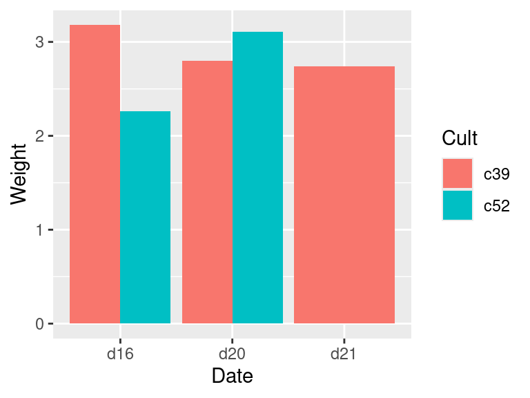
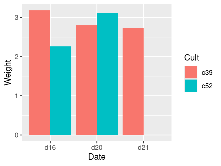
Figure 15.3: Bar graph with a missing combination (left); With missing combination filled (right)
When we used complete(), it filled in the missing combinations with NA. It’s possible to fill with a different value, with the fill parameter. See ?complete for more information.