4.6 Making a Graph with a Shaded Area
4.6.2 Solution
Use geom_area() to get a shaded area, as in Figure 4.17:
# Convert the sunspot.year data set into a data frame for this example
sunspotyear <- data.frame(
    Year     = as.numeric(time(sunspot.year)),
    Sunspots = as.numeric(sunspot.year)
  )

ggplot(sunspotyear, aes(x = Year, y = Sunspots)) +
  geom_area()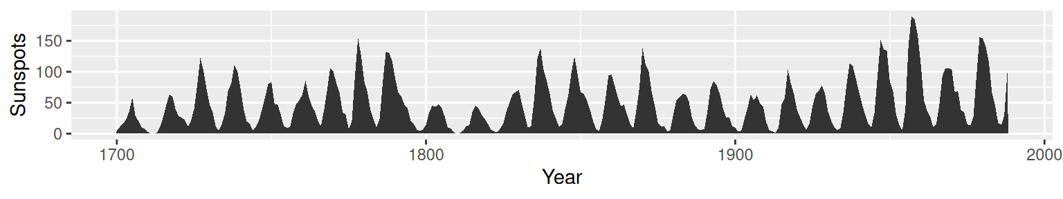
Figure 4.17: Graph with a shaded area
4.6.3 Discussion
By default, the area will be filled with a very dark grey and will have no outline. The color can be changed by setting fill. In the following example, we’ll set it to "blue", and we’ll also make it 80% transparent by setting alpha to 0.2. This makes it possible to see the grid lines through the area, as shown in Figure 4.18. We’ll also add an outline, by setting colour:
ggplot(sunspotyear, aes(x = Year, y = Sunspots)) +
  geom_area(colour = "black", fill = "blue", alpha = .2)
Figure 4.18: Graph with a semitransparent shaded area and an outline
Having an outline around the entire area might not be desirable, because it puts a vertical line at the beginning and end of the shaded area, as well as one along the bottom. To avoid this issue, we can draw the area without an outline (by not specifying colour), and then layer a geom_line() on top, as shown in Figure 4.19:
ggplot(sunspotyear, aes(x = Year, y = Sunspots)) +
  geom_area(fill = "blue", alpha = .2) +
  geom_line()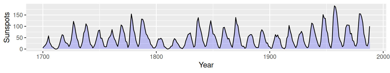
Figure 4.19: Line graph with a line just on top, using geom_line()
4.6.4 See Also
See Chapter 12 for more on choosing colors.