15.16 Calculating New Columns by Groups
15.16.1 Problem
You want to create new columns that are the result of calculations performed on groups of data, as specified by a grouping column.
15.16.2 Solution
Use group_by() from the dplyr package to specify the grouping variable, and then specify the operations in mutate():
library(MASS)  # Load MASS for the cabbages data set
library(dplyr)

cabbages %>%
  group_by(Cult) %>%
  mutate(DevWt = HeadWt - mean(HeadWt))
#> # A tibble: 60 × 5
#> # Groups:   Cult [2]
#>   Cult  Date  HeadWt  VitC  DevWt
#>   <fct> <fct>  <dbl> <int>  <dbl>
#> 1 c39   d16      2.5    51 -0.407
#> 2 c39   d16      2.2    55 -0.707
#> 3 c39   d16      3.1    45  0.193
#> 4 c39   d16      4.3    42  1.39
#> 5 c39   d16      2.5    53 -0.407
#> 6 c39   d16      4.3    50  1.39
#> # ℹ 54 more rows
This returns a new data frame, so if you want to replace the original variable, you will need to save the result over it.
15.16.3 Discussion
Let’s take a closer look at the cabbages data set. It has two grouping variables (factors): Cult, which has levels c39 and c52, and Date, which has levels d16, d20, and d21. It also has two measured numeric variables, HeadWt and VitC:
cabbages
#>    Cult Date HeadWt VitC
#> 1   c39  d16    2.5   51
#> 2   c39  d16    2.2   55
#>  ...<56 more rows>...
#> 59  c52  d21    1.5   66
#> 60  c52  d21    1.6   72
Suppose we want to find, for each case, the deviation of HeadWt from the overall mean. All we have to do is take the overall mean and subtract it from the observed value for each case:
mutate(cabbages, DevWt = HeadWt - mean(HeadWt))
#>    Cult Date HeadWt VitC       DevWt
#> 1   c39  d16    2.5   51 -0.09333333
#> 2   c39  d16    2.2   55 -0.39333333
#>  ...<56 more rows>...
#> 59  c52  d21    1.5   66 -1.09333333
#> 60  c52  d21    1.6   72 -0.99333333
You’ll often want to do separate operations like this for each group, where the groups are specified by one or more grouping variables. Suppose, for example, we want to normalize the data within each group by finding the deviation of each case from the mean within the group, where the groups are specified by Cult. In these cases, we can use group_by() and mutate() together:
First it groups cabbages based on the value of Cult. There are two levels of Cult, c39 and c52. It then applies the mutate() function to each data frame.
The before and after results are shown in Figure 15.2:
# The data before normalizing
ggplot(cb, aes(x = Cult, y = HeadWt)) +
  geom_boxplot()

# After normalizing
ggplot(cb, aes(x = Cult, y = DevWt)) +
  geom_boxplot()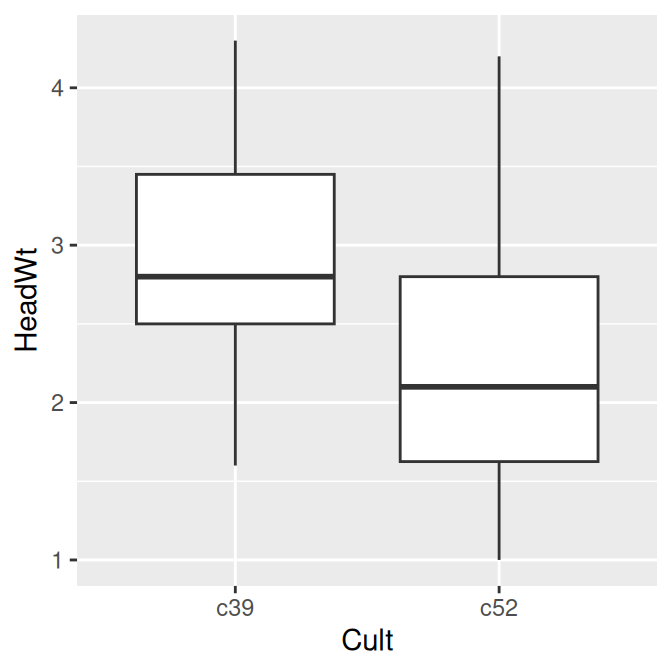
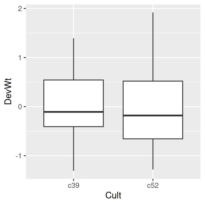
Figure 15.2: Before normalizing (left); After normalizing (right)
You can also group the data frame on multiple variables and perform operations on multiple variables. The following code groups the data by Cult and Date, forming a group for each distinct combination of the two variables. After forming these groups, the code will calculate the deviation of HeadWt and VitC from the mean of each group:
cabbages %>%
  group_by(Cult, Date) %>%
  mutate(
    DevWt = HeadWt - mean(HeadWt),
    DevVitC = VitC - mean(VitC)
  )
#> # A tibble: 60 × 6
#> # Groups:   Cult, Date [6]
#>   Cult  Date  HeadWt  VitC   DevWt DevVitC
#>   <fct> <fct>  <dbl> <int>   <dbl>   <dbl>
#> 1 c39   d16      2.5    51 -0.68     0.700
#> 2 c39   d16      2.2    55 -0.98     4.7
#> 3 c39   d16      3.1    45 -0.0800  -5.3
#> 4 c39   d16      4.3    42  1.12    -8.3
#> 5 c39   d16      2.5    53 -0.68     2.70
#> 6 c39   d16      4.3    50  1.12    -0.300
#> # ℹ 54 more rows
15.16.4 See Also
To summarize data by groups, see Recipe 15.17.