7.8 Adding Annotations to Individual Facets
7.8.2 Solution
Create a new data frame with the faceting variable(s), and a value to use in each facet. Then use geom_text() with the new data frame (Figure 7.17):
# Create the base plot
mpg_plot <- ggplot(mpg, aes(x = displ, y = hwy)) +
  geom_point() +
  facet_grid(. ~ drv)

# A data frame with labels for each facet
f_labels <- data.frame(drv = c("4", "f", "r"), label = c("4wd", "Front", "Rear"))

mpg_plot +
  geom_text(x = 6, y = 40, aes(label = label), data = f_labels)

# If you use annotate(), the label will appear in all facets
mpg_plot +
  annotate("text", x = 6, y = 42, label = "label text")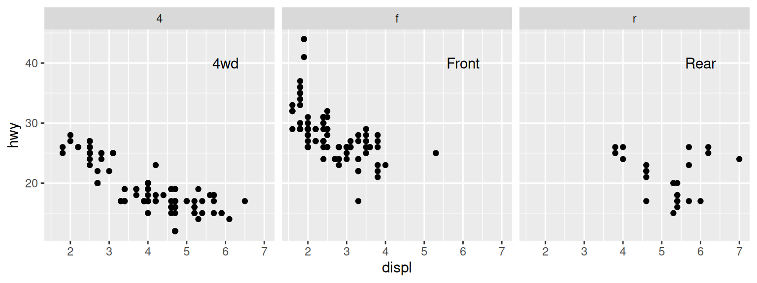

Figure 7.17: Top: different annotations in each facet; bottom: the same annotation in each facet
7.8.3 Discussion
This method can be used to display information about the data in each facet, as shown in Figure 7.18. For example, in each facet we can show linear regression lines, the formula for each line, and the r2 value. To do this, we’ll write a function that takes a data frame and returns another data frame containing a string for a regression equation, and a string for the r2 value. Then we’ll use dplyr’s do() function to apply that function to each group of the data:
# This function returns a data frame with strings representing the regression
# equation, and the r^2 value.
# These strings will be treated as R math expressions
lm_labels <- function(dat) {
  mod <- lm(hwy ~ displ, data = dat)
  formula <- sprintf("italic(y) == %.2f %+.2f * italic(x)",
                     round(coef(mod)[1], 2), round(coef(mod)[2], 2))
  r <- cor(dat$displ, dat$hwy)
  r2 <- sprintf("italic(R^2) == %.2f", r^2)
  data.frame(formula = formula, r2 = r2, stringsAsFactors = FALSE)
}

library(dplyr)
labels <- mpg %>%
  group_by(drv) %>%
  do(lm_labels(.))

labels
#> # A tibble: 3 × 3
#> # Groups:   drv [3]
#>   drv   formula                              r2
#>   <chr> <chr>                                <chr>
#> 1 4     italic(y) == 30.68 -2.88 * italic(x) italic(R^2) == 0.65
#> 2 f     italic(y) == 37.38 -3.60 * italic(x) italic(R^2) == 0.36
#> 3 r     italic(y) == 25.78 -0.92 * italic(x) italic(R^2) == 0.04

# Plot with formula and R^2 values
mpg_plot +
  geom_smooth(method = lm, se = FALSE) +
  geom_text(data = labels, aes(label = formula), x = 3, y = 40, parse = TRUE, hjust = 0) +
  geom_text(x = 3, y = 35, aes(label = r2), data = labels, parse = TRUE, hjust = 0)
#> `geom_smooth()` using formula = 'y ~ x'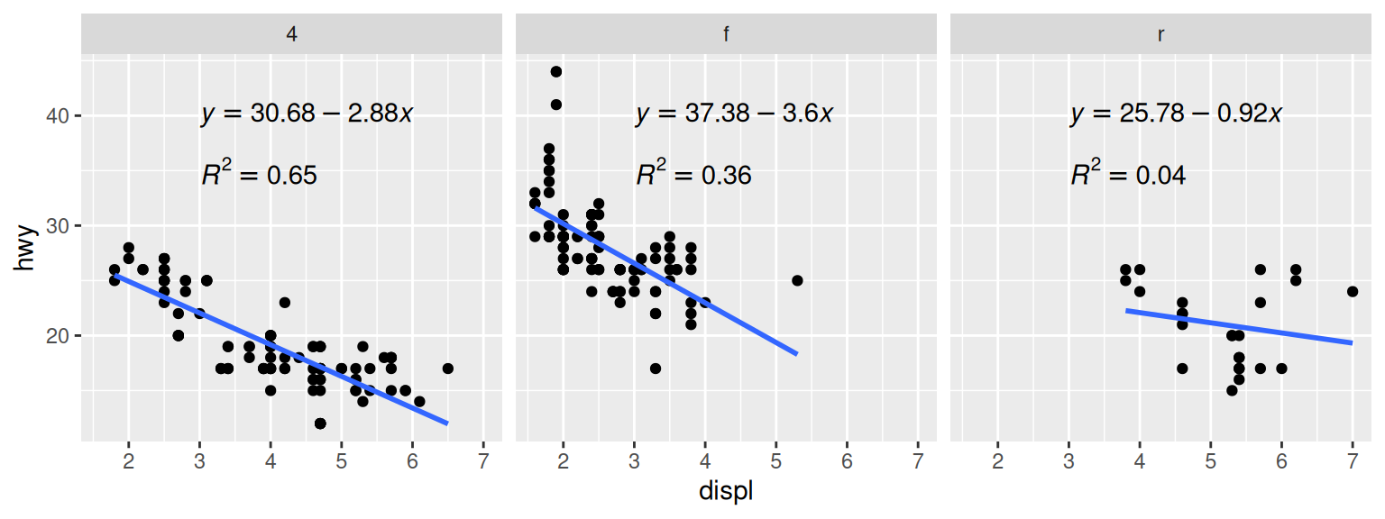
Figure 7.18: Annotations in each facet with information about the data
We needed to write our own function here because generating the linear model and extracting the coefficients requires operating on each subset data frame directly. If you just want to display the r2 values, it’s possible to do something simpler, by using the group_by() and with the summarise() function and then passing additional arguments for summarise():
# Find r^2 values for each group
labels <- mpg %>%
  group_by(drv) %>%
  summarise(r2 = cor(displ, hwy)^2)

labels$r2 <- sprintf("italic(R^2) == %.2f", labels$r2)
labels
#> # A tibble: 3 × 2
#>   drv   r2
#>   <chr> <chr>
#> 1 4     italic(R^2) == 0.65
#> 2 f     italic(R^2) == 0.36
#> 3 r     italic(R^2) == 0.04
Text geoms aren’t the only kind that can be added individually for each facet. Any geom can be used, as long as the input data is structured correctly.