5.1 Making a Basic Scatter Plot

5.1.1 Problem

You want to make a scatter plot using two continuous variables.

5.1.2 Solution

Use geom_point(), and map one variable to x and one variable to y.

We will use the heightweight data set. There are a number of columns in this data set, but we’ll only use two in this example (Figure 5.1):

library(gcookbook) # Load gcookbook for the heightweight data set
library(dplyr)

# Show the head of the two columns we'll use in the plot
heightweight %>%
  select(ageYear, heightIn)
#>     ageYear heightIn
#> 1     11.92     56.3
#> 2     12.92     62.3
#> 3     12.75     63.3
#>  ...<230 more rows>...
#> 235   13.67     61.5
#> 236   13.92     62.0
#> 237   12.58     59.3

ggplot(heightweight, aes(x = ageYear, y = heightIn)) +
  geom_point()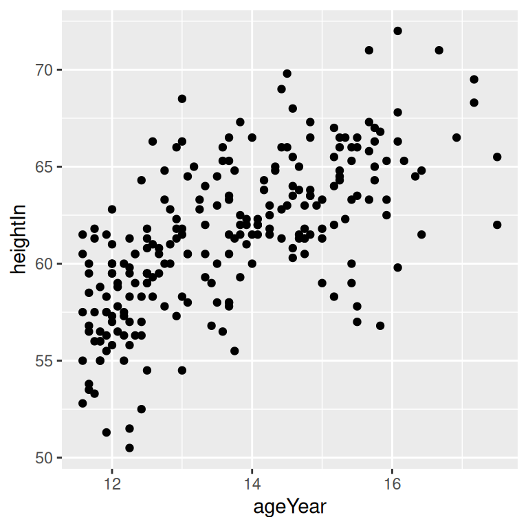

Figure 5.1: A basic scatter plot

5.1.3 Discussion

Instead of points, you can use different shapes for your scatter plot by using the shape aesthetic. A common alternative to the default solid circles (shape #19) is hollow ones (#21), as seen in Figure 5.2 (left):

ggplot(heightweight, aes(x = ageYear, y = heightIn)) +
  geom_point(shape = 21)

The size of the points can be controlled with the size aesthetic. The default value of size is 2 (size = 2). The following code will set size = 1.5 to create smaller points (Figure 5.2, right):

ggplot(heightweight, aes(x = ageYear, y = heightIn)) +
  geom_point(size = 1.5)

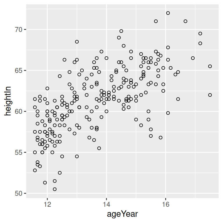
Figure 5.2: Scatter plot with hollow circles (shape 21, left); With smaller points (right)