13.15 Creating a Mosaic Plot
13.15.2 Solution
Use the mosaic() function from the vcd package. For this example we’ll use the USBAdmissions data set, which is a contingency table with three dimensions. We’ll first take a look at the data in a few different ways:
UCBAdmissions
#> , , Dept = A
#>
#>           Gender
#> Admit      Male Female
#>   Admitted  512     89
#>   Rejected  313     19
#>
#> , , Dept = B
#>
#>           Gender
#> Admit      Male Female
#>   Admitted  353     17
#>   Rejected  207      8
#>
#>  ... with 41 more lines of text

# Print a "flat" contingency table
ftable(UCBAdmissions)
#>                 Dept   A   B   C   D   E   F
#> Admit    Gender
#> Admitted Male        512 353 120 138  53  22
#>          Female       89  17 202 131  94  24
#> Rejected Male        313 207 205 279 138 351
#>          Female       19   8 391 244 299 317

dimnames(UCBAdmissions)
#> $Admit
#> [1] "Admitted" "Rejected"
#>
#> $Gender
#> [1] "Male"   "Female"
#>
#> $Dept
#> [1] "A" "B" "C" "D" "E" "F"
The three dimensions are Admit, Gender, and Dept. To visualize the relationships between the variables (Figure 13.27), use mosaic() and pass it a formula with the variables that will be used to split up the data:
# You may need to install first, with install.packages("vcd")
library(vcd)
# Split by Admit, then Gender, then Dept
mosaic( ~ Admit + Gender + Dept, data = UCBAdmissions)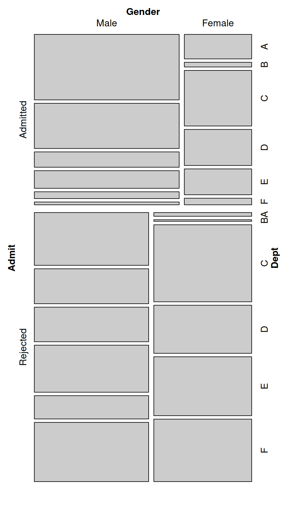
Figure 13.27: Mosaic plot of UC-Berkeley admissions data-the area of each rectangle is proportional to the number of cases in that cell
Notice that mosaic() splits the data in the order in which the variables are provided: first on admission status, then gender, then department. The resulting plot order makes it very clear that more applicants were rejected than admitted. It is also clear that within the admitted group there were many more men than women, while in the rejected group there were approximately the same number of men and women. It is difficult to make comparisons within each department, though. A different variable splitting order may reveal some other interesting information.
Another way of looking at the data is to split first by department, then gender, then admission status, as in Figure 13.28. This makes the admission status the last variable that is partitioned, so that after partitioning by department and gender, the admitted and rejected cells for each group are right next to each other:
mosaic( ~ Dept + Gender + Admit, data = UCBAdmissions,
       highlighting = "Admit", highlighting_fill = c("lightblue", "pink"),
       direction = c("v","h","v"))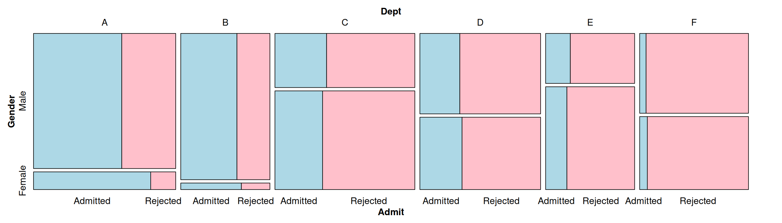
Figure 13.28: Mosaic plot with a different variable splitting order: first department, then gender, then admission status
We also specified a variable to highlight (Admit), and which colors to use in the highlighting.
13.15.3 Discussion
In the preceding example we also specified the direction in which each variable will be split. The first variable, Dept, is split vertically; the second variable, Gender, is split horizontally; and the third variable, Admit, is split vertically. The reason that we chose these directions is because, in this particular example, it makes it easy to compare the male and female groups within each department.
We can also use different splitting directions, as shown in Figure 13.29 and Figure 13.30:
# Another possible set of splitting directions
mosaic( ~ Dept + Gender + Admit, data = UCBAdmissions,
       highlighting = "Admit", highlighting_fill = c("lightblue", "pink"),
       direction = c("v", "v", "h"))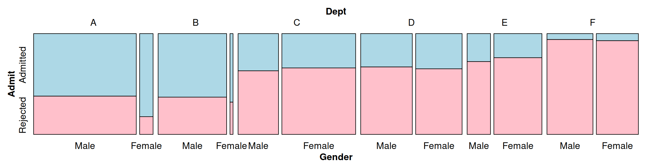
Figure 13.29: Splitting Dept vertically, Gender vertically, and Admit horizontally
# This order makes it difficult to compare male and female
mosaic( ~ Dept + Gender + Admit, data = UCBAdmissions,
       highlighting = "Admit", highlighting_fill = c("lightblue", "pink"),
       direction = c("v", "h", "h"))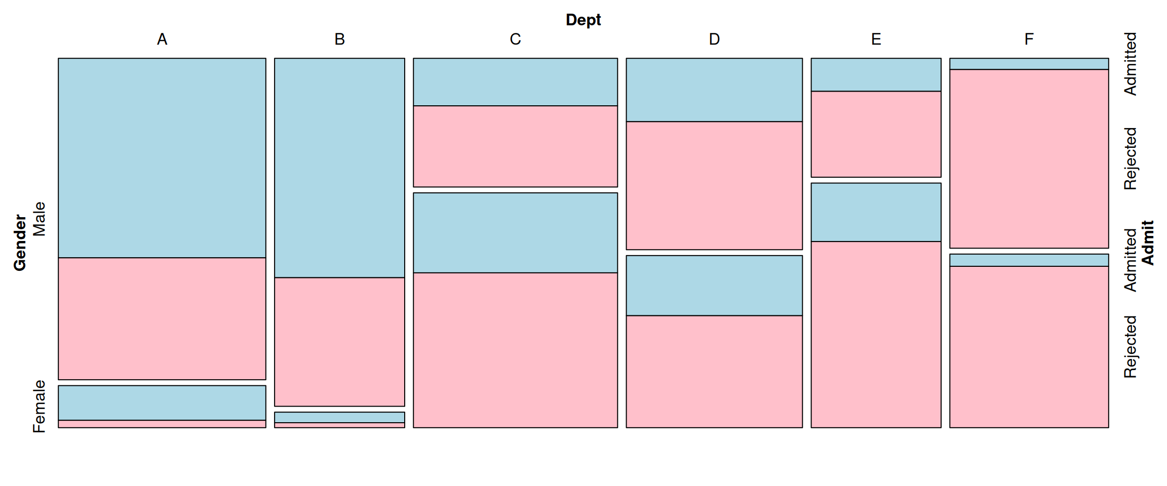
Figure 13.30: Splitting Dept vertically, Gender horizontally, and Admit horizontally
The example here illustrates a classic case of Simpson’s paradox, in which a relationship between variables within subgroups can change (or reverse!) when the groups are combined. The UCBerkeley table contains admissions data from the University of California-Berkeley in 1973. Overall, men were admitted at a higher rate than women, and because of this, the university was sued for gender bias. But when each department was examined separately, it was found that they each had approximately equal admission rates for men and women. The difference in overall admission rates was because women were more likely to apply to competitive departments with lower admission rates.
In Figure 13.28 and Figure 13.29, you can see that within each department, admission rates were approximately equal between men and women. You can also see that departments with higher admission rates (A and B) were very imbalanced in the gender ratio of applicants: far more men applied to these departments than did women. As you can see, partitioning the data in different orders and directions can bring out different aspects of the data. In Figure 13.29, as in Figure 13.28, it’s easy to compare male and female admission rates within each department and across departments. Splitting Dept vertically, Gender horizontally, and Admit horizontally, as in Figure 13.30, makes it difficult to compare male and female admission rates within each department, but it is easy to compare male and female application rates across departments.