13.8 Adding a Prediction Surface to a Three-Dimensional Plot
13.8.2 Solution
First we need to define some utility functions for generating the predicted values from a model object:
# Given a model, predict zvar from xvar and yvar
# Defaults to range of x and y variables, and a 16x16 grid
predictgrid <- function(model, xvar, yvar, zvar, res = 16, type = NULL) {
  # Find the range of the predictor variable. This works for lm and glm
  # and some others, but may require customization for others.
  xrange <- range(model$model[[xvar]])
  yrange <- range(model$model[[yvar]])

  newdata <- expand.grid(x = seq(xrange[1], xrange[2], length.out = res),
                         y = seq(yrange[1], yrange[2], length.out = res))
  names(newdata) <- c(xvar, yvar)
  newdata[[zvar]] <- predict(model, newdata = newdata, type = type)
  newdata
}


# Convert long-style data frame with x, y, and z vars into a list
# with x and y as row/column values, and z as a matrix.
df2mat <- function(p, xvar = NULL, yvar = NULL, zvar = NULL) {
  if (is.null(xvar)) xvar <- names(p)[1]
  if (is.null(yvar)) yvar <- names(p)[2]
  if (is.null(zvar)) zvar <- names(p)[3]

  x <- unique(p[[xvar]])
  y <- unique(p[[yvar]])
  z <- matrix(p[[zvar]], nrow = length(y), ncol = length(x))

  m <- list(x, y, z)
  names(m) <- c(xvar, yvar, zvar)
  m
}

# Function to interleave the elements of two vectors
interleave <- function(v1, v2)  as.vector(rbind(v1,v2))
With these utility functions defined, we can make a linear model from the data and plot it as a mesh along with the data, using the surface3d() function, as shown in Figure 13.17:
library(rgl)

# Make a copy of the data set
m <- mtcars

# Generate a linear model
mod <- lm(mpg ~ wt + disp + wt:disp, data = m)

# Get predicted values of mpg from wt and disp
m$pred_mpg <- predict(mod)

# Get predicted mpg from a grid of wt and disp
mpgrid_df <- predictgrid(mod, "wt", "disp", "mpg")
mpgrid_list <- df2mat(mpgrid_df)

# Make the plot with the data points
plot3d(m$wt, m$disp, m$mpg, type = "s", size = 0.5, lit = FALSE)

# Add the corresponding predicted points (smaller)
spheres3d(m$wt, m$disp, m$pred_mpg, alpha = 0.4, type = "s", size = 0.5, lit = FALSE)

# Add line segments showing the error
segments3d(interleave(m$wt,   m$wt),
           interleave(m$disp, m$disp),
           interleave(m$mpg,  m$pred_mpg),
           alpha = 0.4, col = "red")

# Add the mesh of predicted values
surface3d(mpgrid_list$wt, mpgrid_list$disp, mpgrid_list$mpg,
          alpha = 0.4, front = "lines", back = "lines")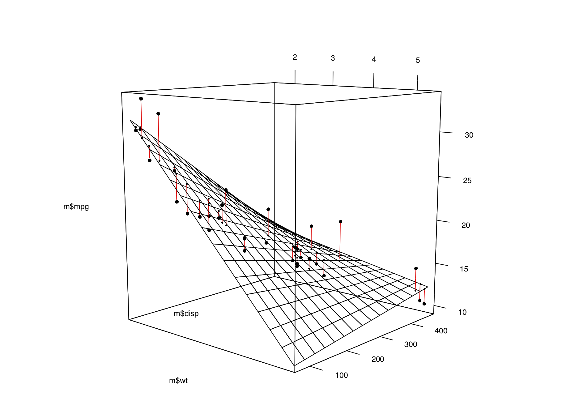
Figure 13.17: A 3D scatter plot with a prediction surface
13.8.3 Discussion
We can tweak the appearance of the graph, as shown in Figure 13.18. We’ll add each of the components of the graph separately:
plot3d(mtcars$wt, mtcars$disp, mtcars$mpg,
       xlab = "", ylab = "", zlab = "",
       axes = FALSE,
       size = .5, type = "s", lit = FALSE)

# Add the corresponding predicted points (smaller)
spheres3d(m$wt, m$disp, m$pred_mpg, alpha = 0.4, type = "s", size = 0.5, lit = FALSE)

# Add line segments showing the error
segments3d(interleave(m$wt,   m$wt),
           interleave(m$disp, m$disp),
           interleave(m$mpg,  m$pred_mpg),
           alpha = 0.4, col = "red")

# Add the mesh of predicted values
surface3d(mpgrid_list$wt, mpgrid_list$disp, mpgrid_list$mpg,
          alpha = 0.4, front = "lines", back = "lines")

# Draw the box
rgl.bbox(color = "grey50",          # grey60 surface and black text
         emission = "grey50",       # emission color is grey50
         xlen = 0, ylen = 0, zlen = 0)  # Don't add tick marks

# Set default color of future objects to black
rgl.material(color = "black")

# Add axes to specific sides. Possible values are "x--", "x-+", "x+-", and "x++".
axes3d(edges = c("x--", "y+-", "z--"),
       ntick = 6,                       # Attempt 6 tick marks on each side
       cex = .75)                       # Smaller font

# Add axis labels. 'line' specifies how far to set the label from the axis.
mtext3d("Weight",       edge = "x--", line = 2)
mtext3d("Displacement", edge = "y+-", line = 3)
mtext3d("MPG",          edge = "z--", line = 3)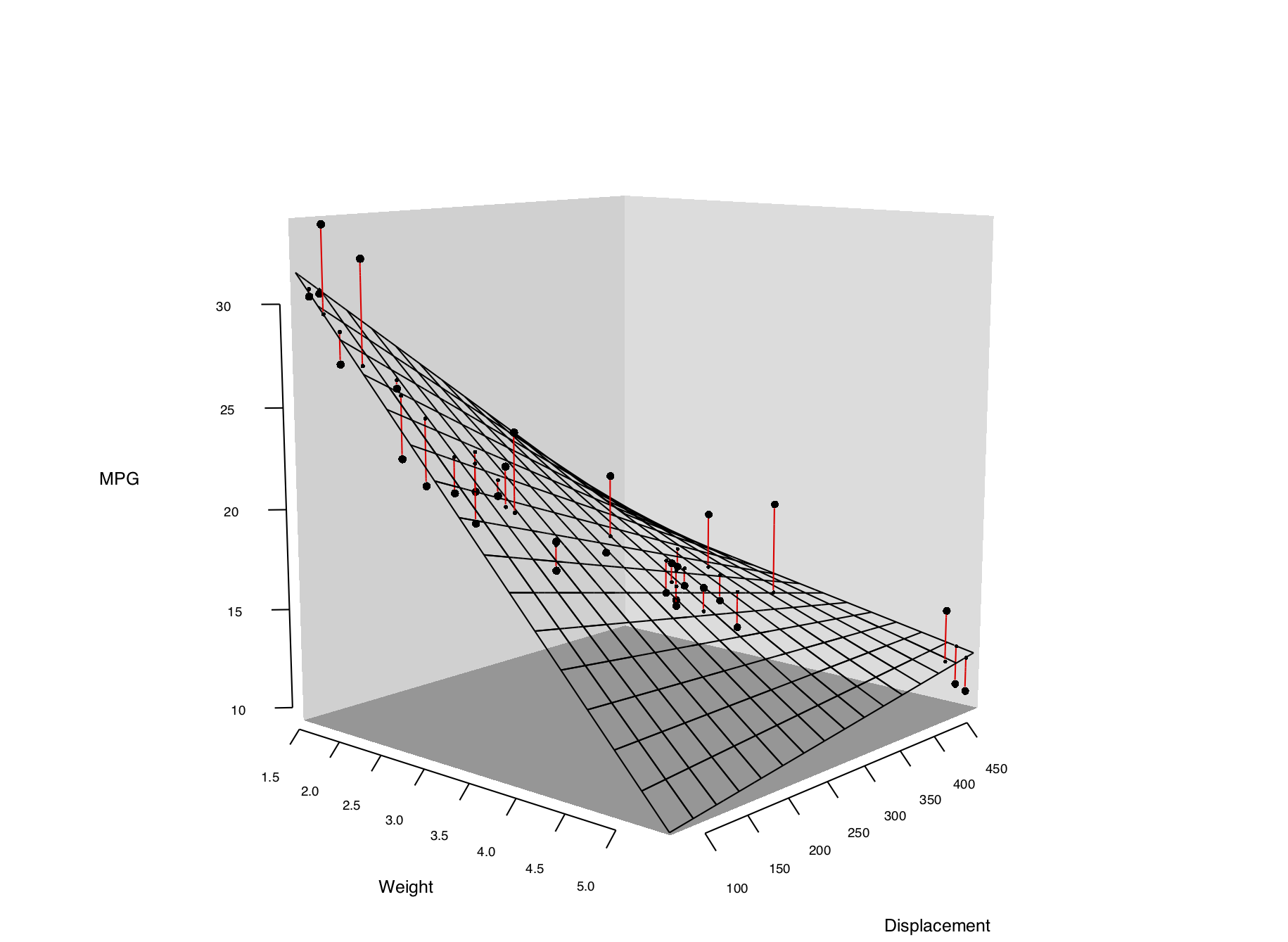
Figure 13.18: Three-dimensional scatter plot with customized appearance