8.8 Changing the Text of Tick Labels
8.8.2 Solution
Consider the scatter plot in Figure 8.15, where height is reported in inches:
library(gcookbook)  # Load gcookbook for the heightweight data set

hw_plot <- ggplot(heightweight, aes(x = ageYear, y = heightIn)) +
  geom_point()

hw_plot
To set arbitrary labels, as in Figure 8.15 (right), pass values to breaks and labels in the scale. One of the labels has a newline (\n) character, which tells ggplot to put a line break there:
hw_plot +
  scale_y_continuous(
    breaks = c(50, 56, 60, 66, 72),
    labels = c("Tiny", "Really\nshort", "Short", "Medium", "Tallish")
  )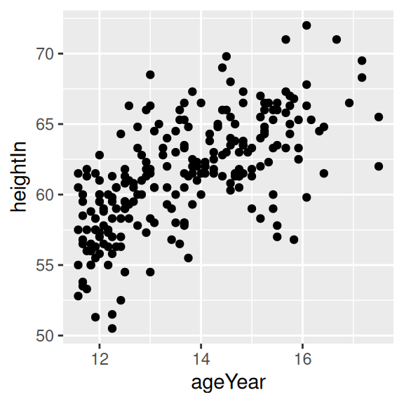
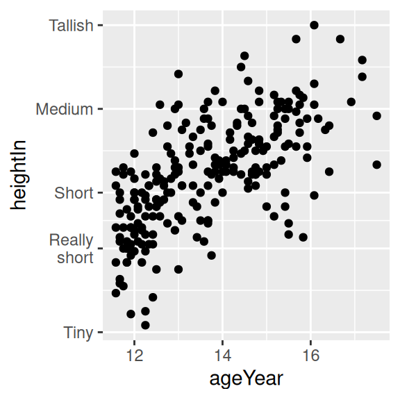
Figure 8.15: Scatter plot with automatic tick labels (left); With manually specified labels on the y-axis (right)
8.8.3 Discussion
Instead of setting completely arbitrary labels, it is more common to have your data stored in one format, while wanting the labels to be displayed in another. We might, for example, want heights to be displayed in feet and inches (like 5’6”) instead of just inches. To do this, we can define a formatter function, which takes in a value and returns the corresponding string. For example, this function will convert inches to feet and inches:
footinch_formatter <- function(x) {
  foot <- floor(x/12)
  inch <- x %% 12
  return(paste(foot, "'", inch, "\"", sep = ""))
}
Here’s what it returns for values 56–64 (the backslashes are there as escape characters, to distinguish the quotes in a string from the quotes that delimit a string):
footinch_formatter(56:64)
#> [1] "4'8\""  "4'9\""  "4'10\"" "4'11\"" "5'0\""  "5'1\""  "5'2\""  "5'3\""
#> [9] "5'4\""
Now we can pass our function to the scale, using the labels parameter (Figure 8.16, left):
Here, the automatic tick marks were placed every five inches, but that looks a little off for this data. We can instead have ggplot set tick marks every four inches, by specifying breaks (Figure 8.16, right):
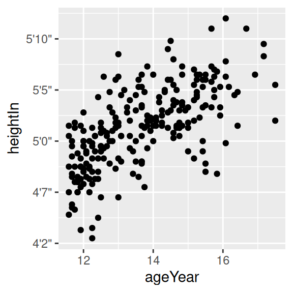
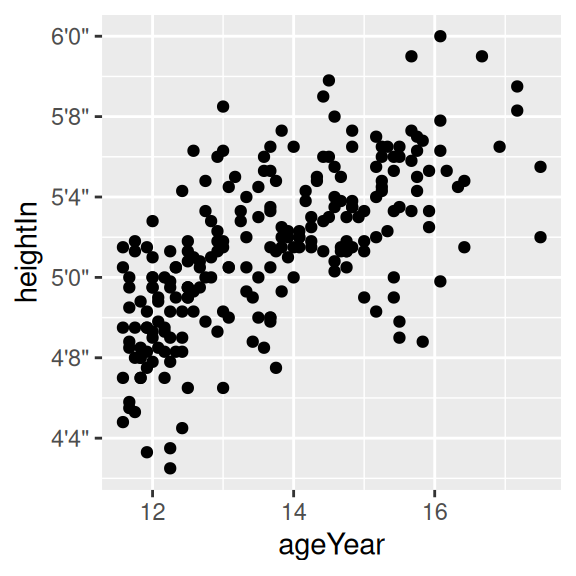
Figure 8.16: Scatter plot with a formatter function (left); With manually specified breaks on the y-axis (right)
Another common task is to convert time measurements to HH:MM:SS format, or something similar. This function will take numeric minutes and convert them to this format, rounding to the nearest second (it can be customized for your particular needs):
timeHMS_formatter <- function(x) {
  h <- floor(x/60)
  m <- floor(x %% 60)
  s <- round(60*(x %% 1))                   # Round to nearest second
  lab <- sprintf("%02d:%02d:%02d", h, m, s) # Format the strings as HH:MM:SS
  lab <- gsub("^00:", "", lab)              # Remove leading 00: if present
  lab <- gsub("^0", "", lab)                # Remove leading 0 if present
  return(lab)
}
Running it on some sample numbers yields:
timeHMS_formatter(c(.33, 50, 51.25, 59.32, 60, 60.1, 130.23))
#> [1] "0:20"    "50:00"   "51:15"   "59:19"   "1:00:00" "1:00:06" "2:10:14"
The scales package, which is installed with ggplot2, comes with some built-in formatting functions:
comma()adds commasto numbers, in the thousand, million, billion, etc. places.dollar()adds a dollar sign and rounds to the nearest cent.percent()multiplies by 100, rounds to the nearest integer, and adds a percent sign.scientific()gives numbers in scientific notation, like3.30e+05, for large and small numbers.
If you want to use these functions, you must first load the scales package, with library(scales).