5.9 Adding Annotations with Model Coefficients
5.9.2 Solution
To add simple text to a plot, simply add an annotation. In this example, we’ll create a linear model and use the predictvals() function defined in Recipe 5.7 to create a prediction line from the model. Then we’ll add an annotation:
library(gcookbook) # Load gcookbook for the heightweight data set

model <- lm(heightIn ~ ageYear, heightweight)
summary(model)
#>
#> Call:
#> lm(formula = heightIn ~ ageYear, data = heightweight)
#>
#> Residuals:
#>     Min      1Q  Median      3Q     Max
#> -8.3517 -1.9006  0.1378  1.9071  8.3371
#>
#> Coefficients:
#>             Estimate Std. Error t value Pr(>|t|)
#> (Intercept)  37.4356     1.8281   20.48   <2e-16 ***
#> ageYear       1.7483     0.1329   13.15   <2e-16 ***
#> ---
#> Signif. codes:  0 '***' 0.001 '**' 0.01 '*' 0.05 '.' 0.1 ' ' 1
#>
#> Residual standard error: 2.989 on 234 degrees of freedom
#> Multiple R-squared:  0.4249, Adjusted R-squared:  0.4225
#> F-statistic: 172.9 on 1 and 234 DF,  p-value: < 2.2e-16
This shows that the r^2 value is 0.4249. We’ll create a graph and manually add the text using annotate() (Figure 5.26):
# First generate prediction data
pred <- predictvals(model, "ageYear", "heightIn")

# Save a base plot
hw_sp <- ggplot(heightweight, aes(x = ageYear, y = heightIn)) +
    geom_point() +
    geom_line(data = pred)

hw_sp +
  annotate("text", x = 16.5, y = 52, label = "r^2=0.42")
Instead of using a plain text string, it’s also possible to enter formulas using R’s math expression syntax, by using parse = TRUE:
hw_sp +
  annotate("text", x = 16.5, y = 52, label = "r^2 == 0.42", parse = TRUE)
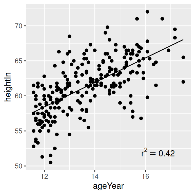
Figure 5.26: Plain text (left); Math expression (right)
5.9.3 Discussion
Text geoms in ggplot do not take expression objects directly; instead, they take character strings that can be turned into expressions with R’s parse() function.
If you use a mathematical expression, the syntax must be correct for the expression to be a valid R expression object. You can test the validity by wrapping the object in the expression() function and seeing if it throws an error (make sure not to use quotes around the expression). In the example here, == is a valid construct in an expression to express equality, but = is not:
expression(r^2 == 0.42) # Valid
expression(r^2 = 0.42)  # Not valid
#> Error: unexpected '=' in "expression(r\^2 ="
It’s possible to automatically extract values from the model object and build an expression using those values. In this example, we’ll create a string which when parsed, yields a valid expression:
# Use sprintf() to construct our string.
# The %.3g and %.2g are replaced with numbers with 3 significant digits and 2
# significant digits, respectively. The numbers are supplied after the string.

eqn <- sprintf(
    "italic(y) == %.3g + %.3g * italic(x) * ',' ~~ italic(r)^2 ~ '=' ~ %.2g",
    coef(model)[1],
    coef(model)[2],
    summary(model)$r.squared
  )

eqn
#> [1] "italic(y) == 37.4 + 1.75 * italic(x) * ',' ~~ italic(r)^2 ~ '=' ~ 0.42"

# Test validity by using parse()
parse(text = eqn)
#> expression(italic(y) == 37.4 + 1.75 * italic(x) * "," ~ ~italic(r)^2 ~
#>     "=" ~ 0.42)
Now that we have the expression string, we can add it to the plot. In this example we’ll put the text in the bottom-right corner, by setting x = Inf and y = -Inf and using horizontal and vertical adjustments so that the text all fits inside the plotting area (Figure 5.27):
hw_sp +
  annotate(
    "text",
    x = Inf, y = -Inf,
    label = eqn, parse = TRUE,
    hjust = 1.1, vjust = -.5
  )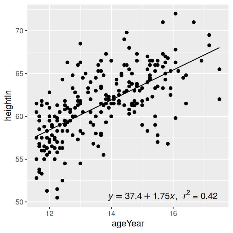
Figure 5.27: Scatter plot with automatically generated expression
5.9.4 See Also
The math expression syntax in R can be a bit tricky. See Recipe 7.2 for more information.