13.18 Creating a Choropleth Map
13.18.1 Problem
You want to create a map with regions that are colored according to variable values.
13.18.2 Solution
Merge the value data with the map data, then map a variable to fill:
# Transform the USArrests data set to the correct format
crimes <- data.frame(state = tolower(rownames(USArrests)), USArrests)
crimes
#>                       state Murder Assault UrbanPop Rape
#> Alabama             alabama   13.2     236       58 21.2
#> Alaska               alaska   10.0     263       48 44.5
#> Arizona             arizona    8.1     294       80 31.0
#>  ...<44 more rows>...
#> West Virginia west virginia    5.7      81       39  9.3
#> Wisconsin         wisconsin    2.6      53       66 10.8
#> Wyoming             wyoming    6.8     161       60 15.6

library(maps) # For map data
states_map <- map_data("state")
# Merge the data sets together
crime_map <- merge(states_map, crimes, by.x = "region", by.y = "state")
# After merging, the order has changed, which would lead to polygons drawn in
# the incorrect order. So, we'll sort the data.
crime_map
#>        region   long  lat group order subregion Murder Assault UrbanPop Rape
#> 1     alabama  -87.5 30.4     1     1      <NA>   13.2     236       58 21.2
#> 2     alabama  -87.5 30.4     1     2      <NA>   13.2     236       58 21.2
#> 3     alabama  -88.0 30.2     1    13      <NA>   13.2     236       58 21.2
#>  ...<15,521 more rows>...
#> 15525 wyoming -107.9 41.0    63 15597      <NA>    6.8     161       60 15.6
#> 15526 wyoming -109.1 41.0    63 15598      <NA>    6.8     161       60 15.6
#> 15527 wyoming -109.1 41.0    63 15599      <NA>    6.8     161       60 15.6

library(dplyr) # For arrange() function
# Sort by group, then order
crime_map <- arrange(crime_map, group, order)
crime_map
#>        region   long  lat group order subregion Murder Assault UrbanPop Rape
#> 1     alabama  -87.5 30.4     1     1      <NA>   13.2     236       58 21.2
#> 2     alabama  -87.5 30.4     1     2      <NA>   13.2     236       58 21.2
#> 3     alabama  -87.5 30.4     1     3      <NA>   13.2     236       58 21.2
#>  ...<15,521 more rows>...
#> 15525 wyoming -107.9 41.0    63 15597      <NA>    6.8     161       60 15.6
#> 15526 wyoming -109.1 41.0    63 15598      <NA>    6.8     161       60 15.6
#> 15527 wyoming -109.1 41.0    63 15599      <NA>    6.8     161       60 15.6
Once the data is in the correct format, it can be plotted (Figure 13.35), mapping one of the columns with data values to fill:
ggplot(crime_map, aes(x = long, y = lat, group = group, fill = Assault)) +
  geom_polygon(colour = "black") +
  coord_map("polyconic")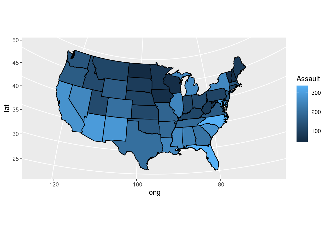
Figure 13.35: A map with a variable mapped to fill
13.18.3 Discussion
The preceding example used the default color scale, which goes from dark to light blue. If you want to show how the values diverge from some middle value, you can use scale_fill_gradient2(), or scale_fill_viridis_c() as shown in Figure 13.36:
# Create a base plot
crime_p <- ggplot(crimes, aes(map_id = state, fill = Assault)) +
  geom_map(map = states_map, colour = "black") +
  expand_limits(x = states_map$long, y = states_map$lat) +
  coord_map("polyconic")

crime_p +
  scale_fill_gradient2(low = "#559999", mid = "grey90", high = "#BB650B",
                       midpoint = median(crimes$Assault))

crime_p +
    scale_fill_viridis_c()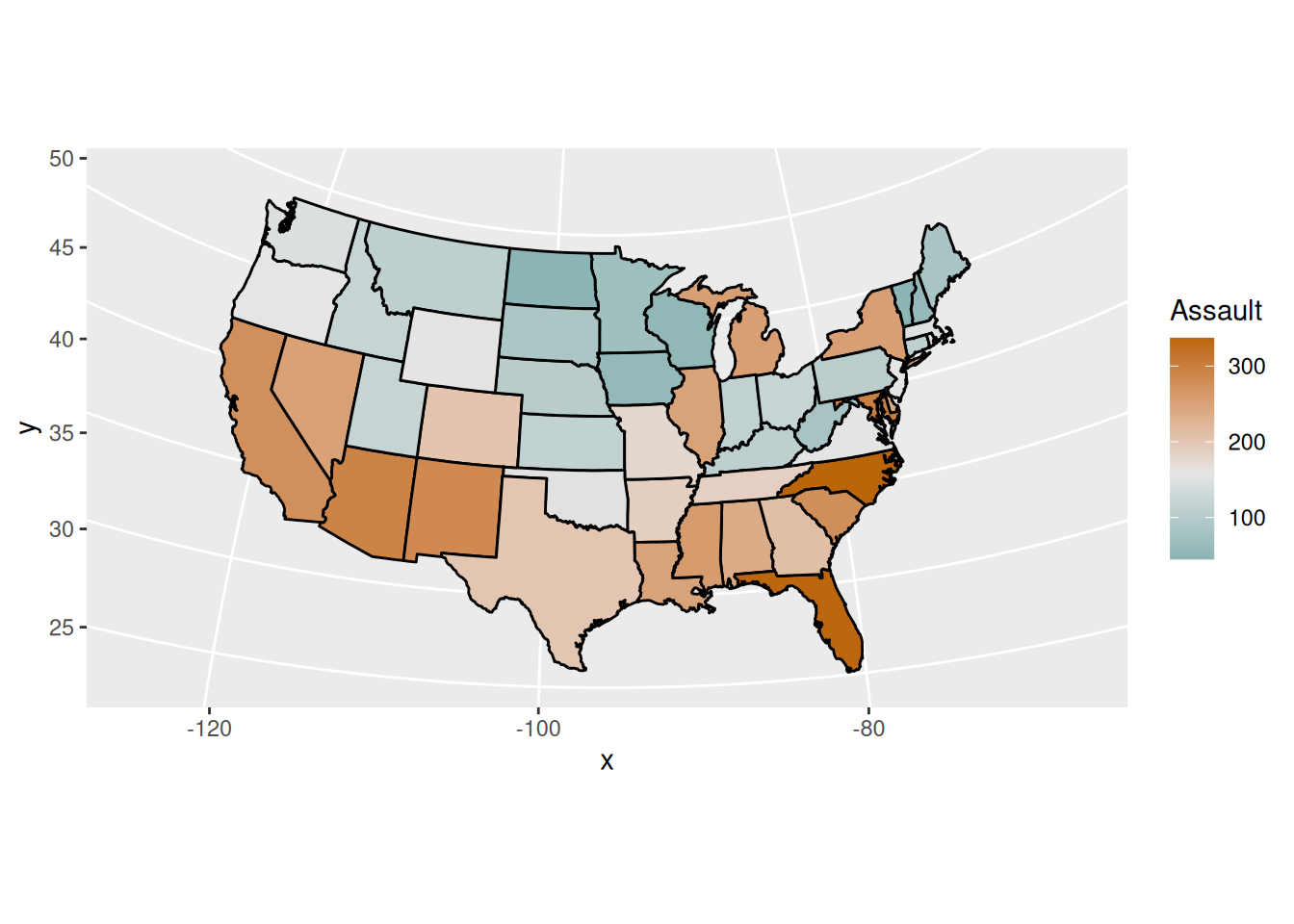
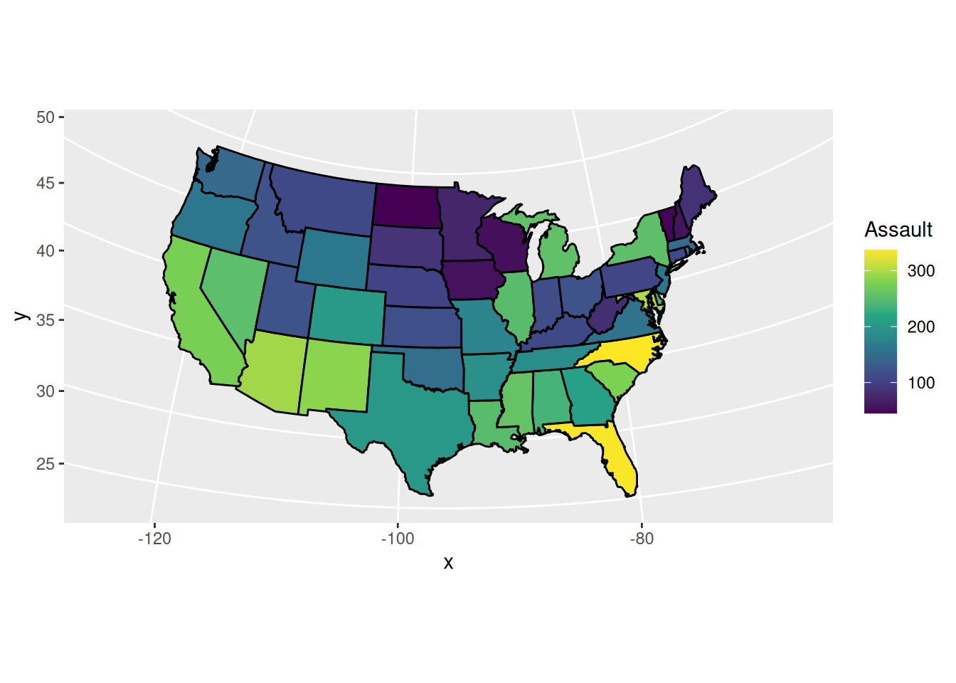
Figure 13.36: With a diverging color scale
The previous example mapped continuous values to fill, but we could just as well use discrete values. It’s sometimes easier to interpret the data if the values are discretized. For example, we can categorize the values into quantiles and show those quantiles, as in Figure 13.37:
# Find the quantile bounds
qa <- quantile(crimes$Assault, c(0, 0.2, 0.4, 0.6, 0.8, 1.0))
qa
#>    0%   20%   40%   60%   80%  100%
#>  45.0  98.8 135.0 188.8 254.2 337.0

# Add a column of the quantile category
crimes$Assault_q <- cut(crimes$Assault, qa,
                        labels = c("0-20%", "20-40%", "40-60%", "60-80%", "80-100%"),
                        include.lowest = TRUE)
crimes
#>                       state Murder Assault UrbanPop Rape Assault_q
#> Alabama             alabama   13.2     236       58 21.2    60-80%
#> Alaska               alaska   10.0     263       48 44.5   80-100%
#> Arizona             arizona    8.1     294       80 31.0   80-100%
#>  ...<44 more rows>...
#> West Virginia west virginia    5.7      81       39  9.3     0-20%
#> Wisconsin         wisconsin    2.6      53       66 10.8     0-20%
#> Wyoming             wyoming    6.8     161       60 15.6    40-60%
# Generate a discrete color palette with 5 values
pal <- colorRampPalette(c("#559999", "grey80", "#BB650B"))(5)
pal
#> [1] "#559999" "#90B2B2" "#CCCCCC" "#C3986B" "#BB650B"

ggplot(crimes, aes(map_id = state, fill = Assault_q)) +
  geom_map(map = states_map, colour = "black") +
  scale_fill_manual(values = pal) +
  expand_limits(x = states_map$long, y = states_map$lat) +
  coord_map("polyconic") +
  labs(fill = "Assault Rate\nPercentile")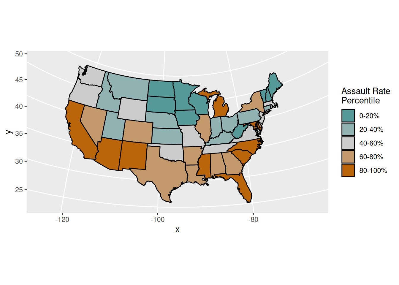
Figure 13.37: Choropleth map with discretized data
Another way to make a choropleth, but without needing to merge the map data with the value data, is to use geom_map(). As of this writing, this will render maps faster than the method just described.
For this method, the map data frame must have columns named lat, long, and region. In the value data frame, there must be a column that is matched to the region column in the map data frame, and this column is specified by mapping it to the map_id aesthetic. For example, this code will have the same output as the first example (Figure 13.35):
# The 'state' column in the crimes data is to be matched to the 'region' column
# in the states_map data
ggplot(crimes, aes(map_id = state, fill = Assault)) +
  geom_map(map = states_map) +
  expand_limits(x = states_map$long, y = states_map$lat) +
  coord_map("polyconic")
Notice that we also needed to use expand_limits(). This is because unlike most geoms, geom_map() doesn’t automatically set the x and y limits; the use of expand_limits() makes it include those x and y values. (Another way to accomplish the same result is to use ylim() and xlim().)