5.4 Mapping a Continuous Variable to Color or Size
5.4.2 Solution
Map the continuous variable to size or colour. We will use the heightweight data set for this example. There are many columns in this data set, but we’ll only use four of them in this example:
library(gcookbook) # Load gcookbook for the heightweight data set

# Show the head of the four columns we'll use
heightweight %>%
  select(sex, ageYear, heightIn, weightLb)
#>     sex ageYear heightIn weightLb
#> 1     f   11.92     56.3     85.0
#> 2     f   12.92     62.3    105.0
#> 3     f   12.75     63.3    108.0
#>  ...<230 more rows>...
#> 235   m   13.67     61.5    140.0
#> 236   m   13.92     62.0    107.5
#> 237   m   12.58     59.3     87.0
The basic scatter plot in Recipe 5.1 shows the relationship between the continuous variables ageYear and heightIn. We can represent a third continuous variable, weightLb, by mapping this variable to another aesthetic property, such as colour or size (Figure 5.8:
ggplot(heightweight, aes(x = ageYear, y = heightIn, colour = weightLb)) +
  geom_point()

ggplot(heightweight, aes(x = ageYear, y = heightIn, size = weightLb)) +
  geom_point()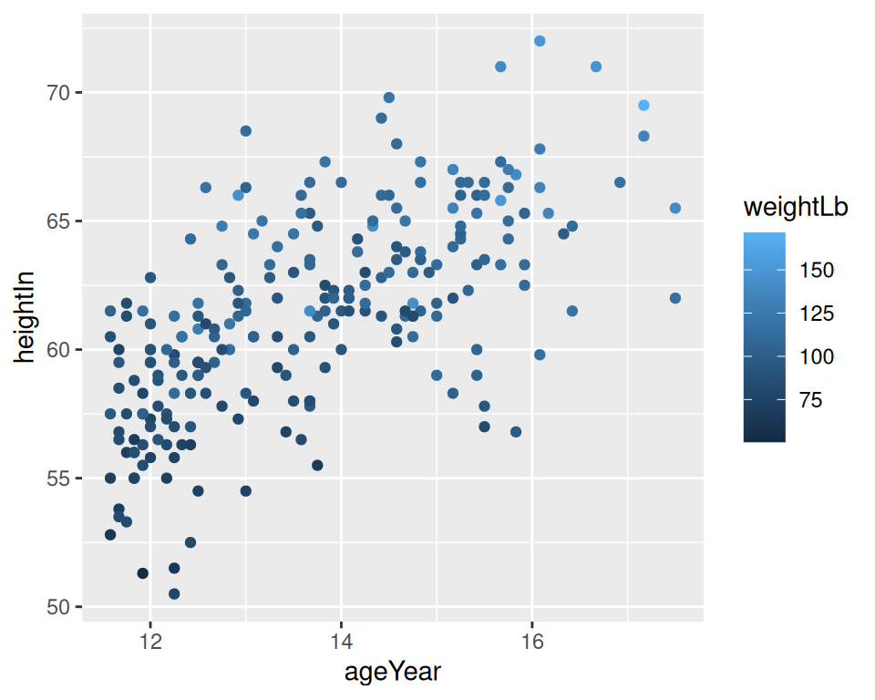

Figure 5.8: A continuous variable mapped to colour (left); Mapped to size (right)
5.4.3 Discussion
A basic scatter plot shows the relationship between two continuous variables: one mapped to the x-axis, and one to the y-axis. When there are more than two continuous variables, these additional variables must be mapped to other aesthetics, like size and color.
Humans can easily perceive small differences in spatial position, so we can interpret the variables mapped to x and y coordinates with high precision. Humans aren’t as good at perceiving small differences in size and color though, so we will interpret variables mapped to these aesthetic attributes with much lower precision. Therefore, when you map a variable to size or color, make sure it is a variable where high precision is not very important for correctly intepreting the data.
There is another consideration when mapping a variable to size, which is that the results can be perceptually misleading. While the largest dots in Figure 5.8 are about 36 times the size of the smallest ones, they are only supposed to represent about 3.5 times the weight of the smallest dots.
This relative misrepresentation of size happens because the default values in ggplot2 for the diameter of points ranges from 1 to 6mm, regardless of the actual data values. For example, if the data values range from 0 to 10, the smallest value of 0 will be represented on the plot with a point that is 1mm wide, while the largest value of 10 will be represented on the plot with a point that is 6mm wide. Similarly, if the data values range from 100 to 110, the smallest value of 100 will still be represented by a point that is 1mm wide, and the largest value of 110 will be represented by a point that is 6mm wide. Thus regardless of the actual data values, the largest point will have a diameter that is 6 times the diameter of the smallest point, and will be 36 times the area.
If it is important for the size of the points to accurately reflect the proportional differences of your data values, you should first decide if you want the diameter of the points to represent the data values, or if you want to area of the points to represent the data values. Figure 5.9 shows the difference between these representations.
range(heightweight$weightLb)
#> [1]  50.5 171.5
size_range <- range(heightweight$weightLb) / max(heightweight$weightLb) *  6
size_range
#> [1] 1.766764 6.000000

ggplot(heightweight, aes(x = ageYear, y = heightIn, size = weightLb)) +
  geom_point() +
  scale_size_continuous(range = size_range)

ggplot(heightweight, aes(x = ageYear, y = heightIn, size = weightLb)) +
  geom_point() +
  scale_size_area()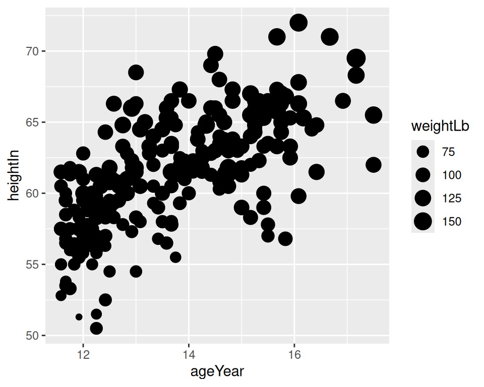

Figure 5.9: Value mapped to diameter of points (left); Value mapped to area of points (right)
See Recipe 5.12 for details on making the area of points proportional to the data values.
When it comes to color, there are actually two aesthetic attributes that can be used: color and fill. You will use color for most point shapes. However, shapes 21–25 have an outline with a solid region in the middle where the color is controlled by fill. These outlined shapes can be useful when using a color scale with light colors as in Figure 5.10, because the outline sets the shapes off from the background. In this example, we also set the fill gradient to go from black to white and make the points larger so that the fill is easier to see:
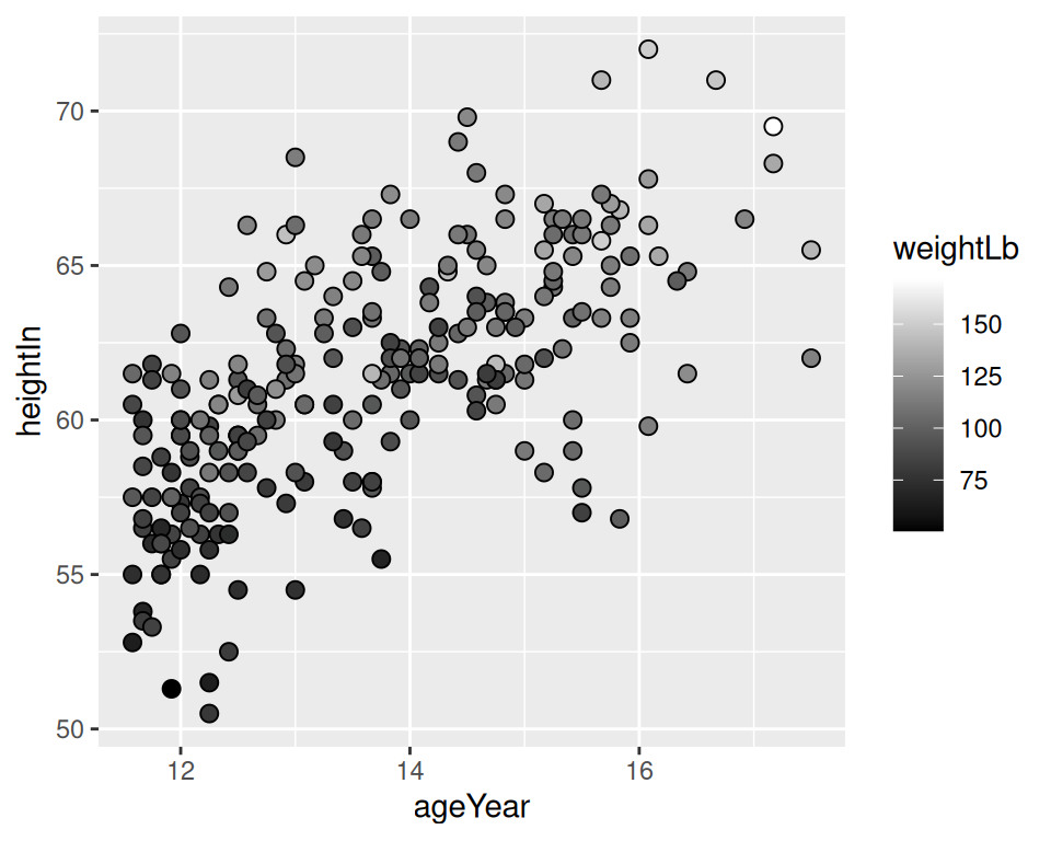
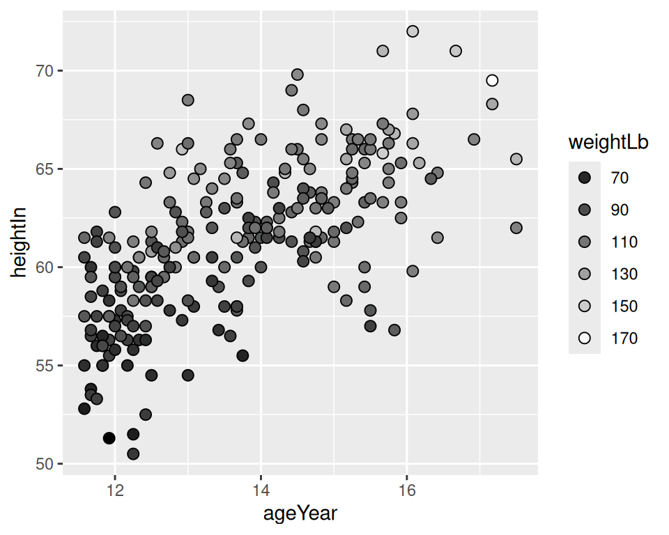
Figure 5.10: Outlined points with a continuous variable mapped to fill (left); With a discrete legend instead of continuous colorbar (right)
Mapping a continuous variable to an aesthetic doesn’t prevent us from mapping a categorical variable to other aesthetics. In Figure 5.11, we’ll map weightLb to size, and also map sex to color. Because there is a fair amount of overplotting (where the points overlap), we’ll make the points 50% transparent by setting alpha = .5. We’ll also use scale_size_area() to make the area of the points proportional to the data values (see Recipe 5.12), and manually change the color palette:
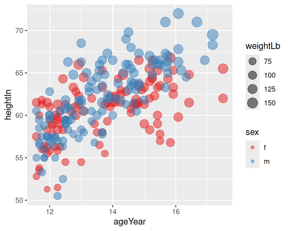
Figure 5.11: Continuous variable mapped to size and categorical variable mapped to colour
When a variable is mapped to size, it’s a good idea to not map a variable to shape. This is because it is difficult to compare the sizes of different shapes; for example, a size 4 triangle could appear larger than a size 3.5 circle. Also, some of the shapes really are different sizes: shapes 16 and 19 are both circles, but at any given numeric size, shape 19 circles are visually larger than shape 16 circles.